Detecting signatures of selection using KLFDAPC
Xinghu Qin
27/10/2020
Source:vignettes/Genome_scan_KLFDAPC.Rmd
Genome_scan_KLFDAPC.RmdKLFDAPC for detection of natural selection
KLFDAPC has multiple advantages over the linear inference and linear discriminant analysis. The population structure inferred using KLFDAPC rectifies the limitation of linear population structure. Thereby, KLFDAPC could be helpful for correcting the genetic gradients (population stratification) in many aspects of population genetic studies, such as correction for geographic genetic structure in genome scan for detecting loci involved in adaptation, and in GWAS for identifying the signatures related to diseases or complex traits. We demonstrate an example using KLFDAPC to detect signatures related to local adaptation. In what follows, we illustrate the step-by-step implementation of genome scan using KLFDAPC.
In this vignette, we use a common implementation similar to PCA-based genome scan that reported by Patterson, N.,et al. 2006 and Luu, K., et al. 2017. However, in this implementation, the loci are weighted by correlation coefficients. We recommended users using more sophisticated implementation with high performance, such as DeepGenomeScan (Qin,X. et al. 2020).
Install packages and dependences
if (!requireNamespace("BiocManager", quietly=TRUE))
    install.packages("BiocManager")

if (!requireNamespace("SNPRelate", quietly=TRUE))
BiocManager::install("SNPRelate")

if (!requireNamespace("KLFDAPC", quietly=TRUE))
devtools::install_github("xinghuq/KLFDAPC")

if (!requireNamespace("DA", quietly=TRUE))
devtools::install_github("xinghuq/DA")
Our package uses the high performance parallel computation processed with SNPRelate (Zheng et al., 2012). It is written by C++, and the data is stored in an efficient format, snpGDS format.
Preparing data
In this vignette, We use the human HapMap data (https://www.genome.gov/10001688/international-hapmap-project) to show how to detect loci involved in adaptation using KLFDAPC.
Data preparation, we use the data that have already in GDS format stored in the library.
# Open the GDS file
genofile <- snpgdsOpen(snpgdsExampleFileName())
# Get sample id
sample.id <- read.gdsn(index.gdsn(genofile, "sample.id"))
# Get population information

pop_code <- read.gdsn(index.gdsn(genofile, "sample.annot/pop.group"))

# assume the order of sample IDs is as the same as population codes

pop_code <- read.gdsn(index.gdsn(genofile, path="sample.annot/pop.group"))
pop_code=factor(pop_code,levels=unique(pop_code))
table(pop_code)

set.seed(1000)

# fliter LD thresholds for sensitivity analysis
snpset <- snpgdsLDpruning(genofile, ld.threshold=0.2)

# Get all selected snp id
snpset.id <- unlist(unname(snpset))

head(snpset.id)

snpgdsClose(genofile)
# pop_code
# YRI CEU HCB JPT
#  93  92  47  47
# SNP pruning based on LD:
# Excluding 365 SNPs on non-autosomes
# Excluding 1 SNP (monomorphic: TRUE, MAF: NaN, missing rate: NaN)
# Working space: 279 samples, 8,722 SNPs
#     using 1 (CPU) core
#     sliding window: 500,000 basepairs, Inf SNPs
#     |LD| threshold: 0.2
#     method: composite
# Chromosome 1: 76.12%, 545/716
# Chromosome 2: 72.78%, 540/742
# Chromosome 3: 74.71%, 455/609
# Chromosome 4: 73.49%, 413/562
# Chromosome 5: 76.86%, 435/566
# Chromosome 6: 75.75%, 428/565
# Chromosome 7: 75.42%, 356/472
# Chromosome 8: 71.11%, 347/488
# Chromosome 9: 77.88%, 324/416
# Chromosome 10: 74.12%, 358/483
# Chromosome 11: 77.85%, 348/447
# Chromosome 12: 76.81%, 328/427
# Chromosome 13: 76.16%, 262/344
# Chromosome 14: 76.60%, 216/282
# Chromosome 15: 76.34%, 200/262
# Chromosome 16: 72.66%, 202/278
# Chromosome 17: 73.91%, 153/207
# Chromosome 18: 73.68%, 196/266
# Chromosome 19: 85.00%, 102/120
# Chromosome 20: 71.62%, 164/229
# Chromosome 21: 76.98%, 97/126
# Chromosome 22: 75.86%, 88/116
# 6,557 markers are selected in total.
# [1]  1  2  4  5  7 10
Doing KLFDAPC on genotype data with a Gaussian kernel
We use a Gaussian kernel with sigma =5 to infer the population structure. After we obtain the genetic structure, we then use it to do genome scan.
showfile.gds(closeall=TRUE)
klfdapcfile <- KLFDAPC(snpgdsExampleFileName(), y=pop_code, snp.id=snpset.id,n.pc = 3,kernel=kernlab::rbfdot(sigma = 5), r=5, num.thread=2)
# Warning: package 'klaR' was built under R version 3.6.3
# Make a data.frame
pop_str <- data.frame(sample.id = klfdapcfile$PCA$sample.id,
pop = factor(pop_code)[match(klfdapcfile$PCA$sample.id, sample.id)],
RD1 = klfdapcfile$KLFDAPC$Z[,1], # the first reduced feature
RD2 = klfdapcfile$KLFDAPC$Z[,2], # the second reduced feature
stringsAsFactors = FALSE)
head(pop_str)
rownames(pop_str)=pop_str$sample.id
# Principal Component Analysis (PCA) on genotypes:
# Excluding 2,531 SNPs (non-autosomes or non-selection)
# Excluding 0 SNP (monomorphic: TRUE, MAF: NaN, missing rate: NaN)
# Working space: 279 samples, 6,557 SNPs
# using 2 (CPU) cores
# PCA: the sum of all selected genotypes (0,1,2) = 1828045
# CPU capabilities: Double-Precision SSE2
# Thu Oct 29 00:40:50 2020 (internal increment: 1276)
#
[..................................................] 0%, ETC: ---
[==================================================] 100%, completed, 0s
# Thu Oct 29 00:40:50 2020 Begin (eigenvalues and eigenvectors)
# Thu Oct 29 00:40:50 2020 Done.
# [1] "Doing KLFDAPC"
# sample.id pop RD1 RD2
# 1 NA19152 YRI -53.71177 -19.85460
# 2 NA19139 YRI -55.41972 -19.32379
# 3 NA18912 YRI -49.86350 -22.98661
# 4 NA19160 YRI -58.62539 -22.75500
# 5 NA07034 CEU 79.90126 73.59765
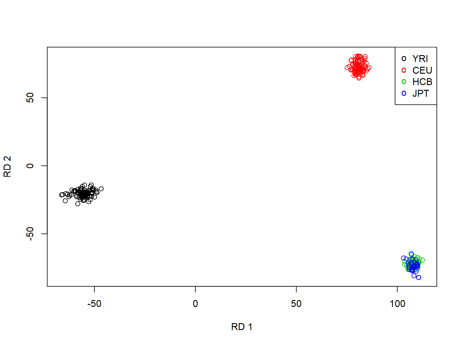
# 6 NA07055 CEU 82.78208 75.75534Visualize the population structure
Project the genetic features onto a plane.
plot(pop_str$RD1, pop_str$RD2, col=as.integer(pop_str$pop), xlab="RD 1", ylab="RD 2")
legend("topright", legend=levels(pop_str$pop), pch="o", col=1:nlevels(pop_str$pop))
Doing genome scan using KLFDAPT
After we choose the genetic features, we then use the genetic features to do genome scan with KLFDAPT.
?KLFDAPT to see the documentation. This genome scan is handeled with a C++ function, which is faster than other implementation. Users can also set the parallel process by changing the paramters of num.threshold.
showfile.gds(closeall=TRUE)
# Get chromosome index
genofile <- snpgdsOpen(snpgdsExampleFileName())
chr <- read.gdsn(index.gdsn(genofile, "snp.chromosome"))
klfdapcmat=as.matrix(pop_str[,-c(1:2)])
### Doing genome scan
### using the correlation to estimate the contribution of SNPs to the pop str (which is the same as PCA does )
klfdapcscanqvalue <- KLFDAPT(klfdapcmat, genofile, n.RD=1:2)
# Warning: package 'robust' was built under R version 3.6.3
# Warning: package 'fit.models' was built under R version 3.6.3
# SNP Correlation:
# Working space: 279 samples, 9088 SNPs
# using 1 (CPU) core
# using the top 2 eigenvectors
# Correlation: the sum of all selected genotypes (0,1,2) = 2553065
# Thu Oct 29 00:40:51 2020 (internal increment: 10216)
#
[..................................................] 0%, ETC: ---
[==================================================] 100%, completed, 0s
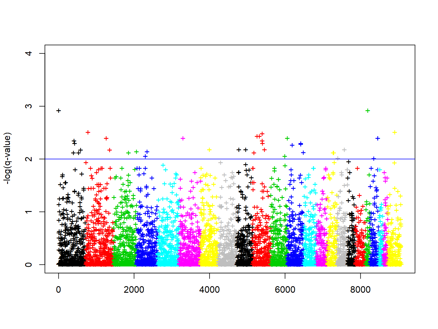
# Thu Oct 29 00:40:51 2020 Done.Plot manhattan plot
###plot manhattan plot
 plot(-log10(klfdapcscanqvalue$q.values$q.values), ylim=c(0,4), xlab="", ylab="-log(q-value)",col=chr, pch="+")
   abline(h=2, col="blue")
Reference
Patterson, N., Price, A. L., & Reich, D. (2006). Population structure and eigenanalysis. PLoS genet, 2(12), e190.
Luu, K., Bazin, E., & Blum, M. G. (2017). pcadapt: an R package to perform genome scans for selection based on principal component analysis. Molecular ecology resources, 17(1), 67-77.
A High-performance Computing Toolset for Relatedness and Principal Component Analysis of SNP Data. Xiuwen Zheng; David Levine; Jess Shen; Stephanie M. Gogarten; Cathy Laurie; Bruce S. Weir. Bioinformatics 2012; doi: 10.1093/bioinformatics/bts606.
R. A. Maronna and R. H. Zamar (2002) Robust estimates of location and dispersion of high-dimensional datasets. Technometrics 44 (4), 307–317.
Wang, J., Zamar, R., Marazzi, A., Yohai, V., Salibian-Barrera, M., Maronna, R., … & Maechler, M. (2017). robust: Port of the S+“Robust Library”. R package version 0.4-18. Available online at: https://CRAN. R-project. org/package= robust.
Qin, X., Chiang, C. W., & Gaggiotti, O. E. (2022). KLFDAPC: a supervised machine learning approach for spatial genetic structure analysis. Briefings in Bioinformatics, 23(4), bbac202.
Zheng X, Levine D, Shen J, Gogarten S, Laurie C, Weir B (2012). A High-performance Computing Toolset for Relatedness and Principal Component Analysis of SNP Data.” Bioinformatics, 28(24), 3326-3328. doi: 10.1093/bioinformatics/bts606.