Population structure of SARS-Cov-2
Xinghu Qin
27/10/2020
Source:vignettes/Population_structure_of_Covid.Rmd
Population_structure_of_Covid.RmdUsing KLFDAPC to infer the population structue of SARS-Cov-2
In this vignette, we demonstrate KLFDAPC for inference of the genetic structure of SARS-Cov-2. We used 3,736 SARS-Cov-2 samples obtained from China National Center for Bioinformation-2019 Novel Coronavirus Resource (2019nCoVR).
The data have been converted to gds file stored in the extdata folder in the package library. As long as you have installed the package, you can get the data using the codes listed below.
library(KLFDAPC)

f <- system.file('extdata',package='KLFDAPC')

infile <- file.path(f, "2019-nCoV_total.gds")
We have ignored the sample origin in this vignette. If you are interested in the details of which countries are they smapled from, you can check the China National Center for Bioinformation-2019 Novel Coronavirus Resource (2019nCoVR) or check the raw data labels. However, here, in this analysis, we just demonstrate how to use KLFDAPC to infer the population structue. We generate random group labels for viruses.
KLFDAPC Analysis with a Gaussian kernel
We use a Gaussian kernel with a sigma = 5 to do the analysis. We filter the SNPs with a missing rate of 0.05, and MAF>0.05, and keep 20 PCs for kernel local discriminant analysis. We then produce the first three genetic features for visualizing the population structure.
# Using Gaussian kernel
# This will take longer than PCA, denpending on the number of samples and n.pcs. We will not show the results here. Users can test on their own clusters
virus_klfdapc=KLFDAPC(infile,y,kernel=kernlab::rbfdot(sigma = 5),r=3,snp.id=NULL, maf=0.05, missing.rate=0.05,n.pc=20,tol=1e-30, num.thread=2,metric = "plain",prior = NULL)
# Warning: package 'klaR' was built under R version 3.6.3
# Warning in FUN(X[[i]], ...): Numerical 0 probability for all classes with
# observation 382
# Warning in FUN(X[[i]], ...): Numerical 0 probability for all classes with
# observation 399
# Warning in FUN(X[[i]], ...): Numerical 0 probability for all classes with
# observation 431
# Warning in FUN(X[[i]], ...): Numerical 0 probability for all classes with
# observation 628
# Warning in FUN(X[[i]], ...): Numerical 0 probability for all classes with
# observation 704
# Warning in FUN(X[[i]], ...): Numerical 0 probability for all classes with
# observation 735
# Warning in FUN(X[[i]], ...): Numerical 0 probability for all classes with
# observation 752
# Warning in FUN(X[[i]], ...): Numerical 0 probability for all classes with
# observation 803
# Warning in FUN(X[[i]], ...): Numerical 0 probability for all classes with
# observation 840
# Warning in FUN(X[[i]], ...): Numerical 0 probability for all classes with
# observation 884
# Warning in FUN(X[[i]], ...): Numerical 0 probability for all classes with
# observation 889
# Warning in FUN(X[[i]], ...): Numerical 0 probability for all classes with
# observation 890
# Warning in FUN(X[[i]], ...): Numerical 0 probability for all classes with
# observation 891
# Warning in FUN(X[[i]], ...): Numerical 0 probability for all classes with
# observation 899
# Warning in FUN(X[[i]], ...): Numerical 0 probability for all classes with
# observation 919
# Warning in FUN(X[[i]], ...): Numerical 0 probability for all classes with
# observation 936
# Warning in FUN(X[[i]], ...): Numerical 0 probability for all classes with
# observation 941
# Warning in FUN(X[[i]], ...): Numerical 0 probability for all classes with
# observation 944
# Warning in FUN(X[[i]], ...): Numerical 0 probability for all classes with
# observation 949
# Warning in FUN(X[[i]], ...): Numerical 0 probability for all classes with
# observation 963
# Warning in FUN(X[[i]], ...): Numerical 0 probability for all classes with
# observation 1097
# Warning in FUN(X[[i]], ...): Numerical 0 probability for all classes with
# observation 1115
# Warning in FUN(X[[i]], ...): Numerical 0 probability for all classes with
# observation 1275
# Warning in FUN(X[[i]], ...): Numerical 0 probability for all classes with
# observation 1289
# Warning in FUN(X[[i]], ...): Numerical 0 probability for all classes with
# observation 1294
# Warning in FUN(X[[i]], ...): Numerical 0 probability for all classes with
# observation 1303
# Warning in FUN(X[[i]], ...): Numerical 0 probability for all classes with
# observation 1304
# Warning in FUN(X[[i]], ...): Numerical 0 probability for all classes with
# observation 1306
# Warning in FUN(X[[i]], ...): Numerical 0 probability for all classes with
# observation 1327
# Warning in FUN(X[[i]], ...): Numerical 0 probability for all classes with
# observation 1336
# Warning in FUN(X[[i]], ...): Numerical 0 probability for all classes with
# observation 1359
# Warning in FUN(X[[i]], ...): Numerical 0 probability for all classes with
# observation 1360
# Warning in FUN(X[[i]], ...): Numerical 0 probability for all classes with
# observation 1475
# Warning in FUN(X[[i]], ...): Numerical 0 probability for all classes with
# observation 1536
# Warning in FUN(X[[i]], ...): Numerical 0 probability for all classes with
# observation 1751
# Warning in FUN(X[[i]], ...): Numerical 0 probability for all classes with
# observation 2289
# Warning in FUN(X[[i]], ...): Numerical 0 probability for all classes with
# observation 2298
# Warning in FUN(X[[i]], ...): Numerical 0 probability for all classes with
# observation 2407
# Warning in FUN(X[[i]], ...): Numerical 0 probability for all classes with
# observation 2443
# Warning in FUN(X[[i]], ...): Numerical 0 probability for all classes with
# observation 2622
# Warning in FUN(X[[i]], ...): Numerical 0 probability for all classes with
# observation 2623
# Warning in FUN(X[[i]], ...): Numerical 0 probability for all classes with
# observation 2624
# Warning in FUN(X[[i]], ...): Numerical 0 probability for all classes with
# observation 2625
# Warning in FUN(X[[i]], ...): Numerical 0 probability for all classes with
# observation 2626
# Warning in FUN(X[[i]], ...): Numerical 0 probability for all classes with
# observation 2631
# Warning in FUN(X[[i]], ...): Numerical 0 probability for all classes with
# observation 3223
# Warning in FUN(X[[i]], ...): Numerical 0 probability for all classes with
# observation 3270
# Warning in FUN(X[[i]], ...): Numerical 0 probability for all classes with
# observation 3335
# Warning in FUN(X[[i]], ...): Numerical 0 probability for all classes with
# observation 3336
# Warning in FUN(X[[i]], ...): Numerical 0 probability for all classes with
# observation 3360
# Warning in FUN(X[[i]], ...): Numerical 0 probability for all classes with
# observation 3364
# Warning in FUN(X[[i]], ...): Numerical 0 probability for all classes with
# observation 3369
# Warning in FUN(X[[i]], ...): Numerical 0 probability for all classes with
# observation 3376
# Warning in FUN(X[[i]], ...): Numerical 0 probability for all classes with
# observation 3377
# Warning in FUN(X[[i]], ...): Numerical 0 probability for all classes with
# observation 3387
# Warning in FUN(X[[i]], ...): Numerical 0 probability for all classes with
# observation 3395
# Warning in FUN(X[[i]], ...): Numerical 0 probability for all classes with
# observation 3403
# Warning in FUN(X[[i]], ...): Numerical 0 probability for all classes with
# observation 3447
# Warning in FUN(X[[i]], ...): Numerical 0 probability for all classes with
# observation 3457
# Warning in FUN(X[[i]], ...): Numerical 0 probability for all classes with
# observation 3596
showfile.gds(closeall=TRUE)
# Principal Component Analysis (PCA) on genotypes:
# Excluding 0 SNP on non-autosomes
# Excluding 153 SNPs (monomorphic: TRUE, MAF: 0.05, missing rate: 0.05)
# Working space: 3,736 samples, 3,065 SNPs
# using 2 (CPU) cores
# PCA: the sum of all selected genotypes (0,1,2) = 11420248
# CPU capabilities: Double-Precision SSE2
# Thu Oct 29 00:40:58 2020 (internal increment: 92)
#
[..................................................] 0%, ETC: ---
[==================================================] 100%, completed, 6s
# Thu Oct 29 00:41:04 2020 Begin (eigenvalues and eigenvectors)
# Thu Oct 29 00:41:29 2020 Done.
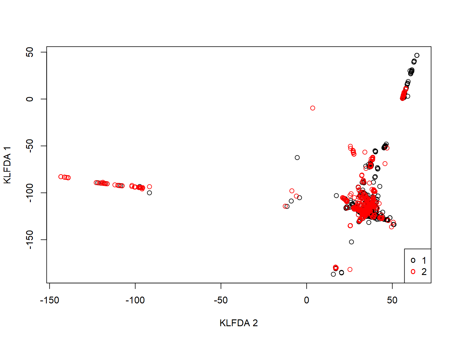
# [1] "Doing KLFDAPC"Plot the population structure of SARS-Cov-2
plot(virus_klfdapc$KLFDAPC$Z[,1], virus_klfdapc$KLFDAPC$Z[,2], col=as.integer(y), xlab="KLFDA 2", ylab="KLFDA 1")
legend("bottomright", legend=levels(y), pch="o", col=1:nlevels(y))
References
Zhao WM, Song SH, Chen ML, et al. The 2019 novel coronavirus resource. Yi Chuan. 2020;42(2):212–221. doi:10.16288/j.yczz.20-030 [PMID: 32102777]
Qin, X. 2020. KLFDAPC: Kernel Local Fisher Discriminant Analysis of Principal Components (KLFDAPC) for large genomic data. R package version 0.2.0.
Qin, X., Chiang, C.W.K., and Gaggiotti, O.E. (2021). Kernel Local Fisher Discriminant Analysis of Principal Components (KLFDAPC) significantly improves the accuracy of predicting geographic origin of individuals. bioRxiv, 2021.2005.2015.444294.