Population structure of Regmap data

KLFDAPC for inference of population structue of Regmap data

In this vignette, we demonstrate KLFDAPC for visualizing populartion structure of Regmap dataset (Arabidopsis thaliana) (Horton,et al., 2012). The reduced features of KLFDAPC retrive the geographic origins of the Arabidopsis thaliana. This is also a tpyical example for recapitulating the geographic origin of individuals using KLFDAPC.

Loading packages into your R environment.


library(KLFDAPC)

library(PCAviz)

library(ggplot2)

library(cowplot)

Load the data

The dataset is already pre-processed data containing the computed PCs of RegMap data. We now load the data and compute the kernel local genetic features.

Load the data and print a summary of the PCs of RegMap data.

data(regmappcs)

### we have to remove the not well represented individuals, which one country only has one individuals.
table(regmappcs$country)

regmapviz=pcaviz(dat = regmappcs)

summary(regmapviz)

### remove unrepresented individuals
regmapviz <- subset(regmapviz,!(country == "AZE" | country == "CPV"| country == "DEN"| country == "GEO"| country == "IND"| country == "LIB"| country == "NOR"| country == "NZL")) 

### 25 countries
regmapviz$data$country=factor(regmapviz$data$country,levels = unique(regmapviz$data$country))

regmapviz1=pcaviz(dat = regmapviz$data)
# 
# AUT AZE BEL CAN CPV CZE DEN ESP FIN FRA GEO GER IND IRL ITA JPN KAZ LIB LTU NED 
#   9   1   4   3   1 154   1  24   4 222   1 100   1   2  12   3   2   1   3  18 
# NOR NZL POL POR ROU RUS SUI SWE TJK  UK UKR UNK USA 
#   1   1   6   6   2  15  10 319   4 185   3   2 187 
# first 4 (of 10) principal components (PCs): 
# # statistics are (s.d.,min,median,max)
# # s.d.=sqrt(eigenvalue) 
#  variable n    stats                 
#  PC1      1307 (NA,-64.7,+0.307,+104)
#  PC2      1307 (NA,-53.8,-2.38,+112) 
#  PC3      1307 (NA,-128,+3.44,+55.8) 
#  PC4      1307 (NA,-70.3,-1.4,+74.3) 
# categorical variables: 
#  variable n    stats                                  
#  region   1227 26 levels, largest=Western Europe (334)
#  country  1307 33 levels, largest=SWE (319)           
# continuous variables: 
# # statistics are (min,median,max) 
#  variable         n    stats             
#  median_intensity 1179 (127,526,1.47e+03)
#  latitude         1302 (-37.8,49.5,65.2) 
#  longitude        1302 (-123,6.19,175)   
# first 4 (of 6) other variables: 
#  variable   n    stats
#  array_id   1307 <NA> 
#  ecotype_id 1307 <NA> 
#  nativename 1307 <NA> 
#  firstname  1307 <NA>

Kernel Local Fisher Discriminant Analysis of Principal Components


### The first 10 PCs, we will produce 3 genetic features for visualization
normalize <- function(x) {
return ((x - min(x)) / (max(x) - min(x)))
}


pcanorm=apply(regmapviz1$data[,12:21], 2, normalize)

reg_kmat <- kmatrixGauss(pcanorm,sigma=10)

reg_klfdapc=KLFDA(reg_kmat, y=regmapviz1$data$country, r=3, knn = 1)

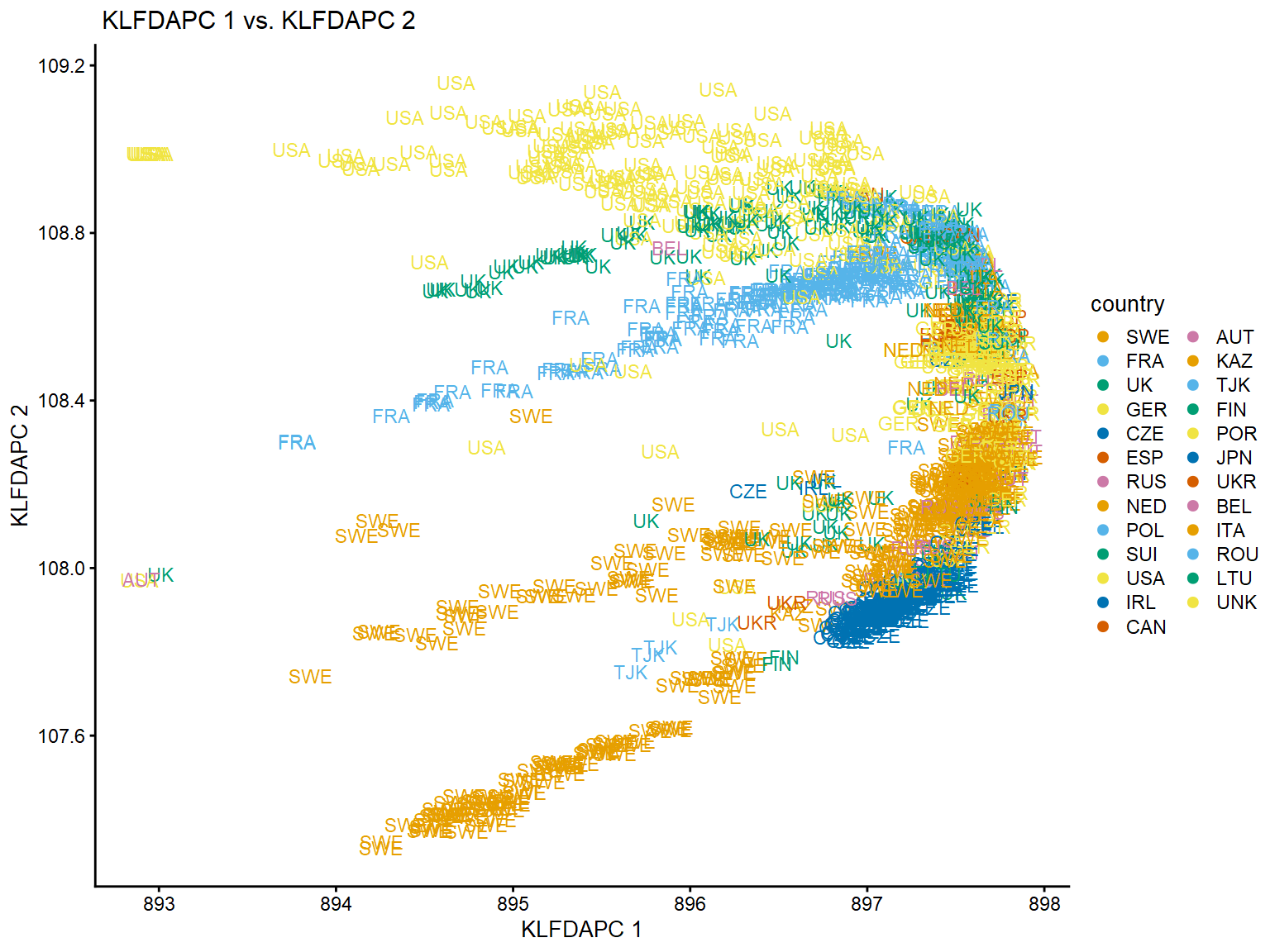
Visualization of the population structure

We can project the the first two genetic features onto the plane, with the samples labeled by the collecting country.


regmapviz1$data$PC1=reg_klfdapc$Z[,1]

regmapviz1$data$PC2=reg_klfdapc$Z[,2]

plot(regmapviz1,coord=c("PC1","PC2"),group =NULL,draw.points =FALSE,label = "country",plot.title=" KLFDAPC 1 vs. KLFDAPC 2")+xlab("KLFDAPC 1")+ylab("KLFDAPC 2")

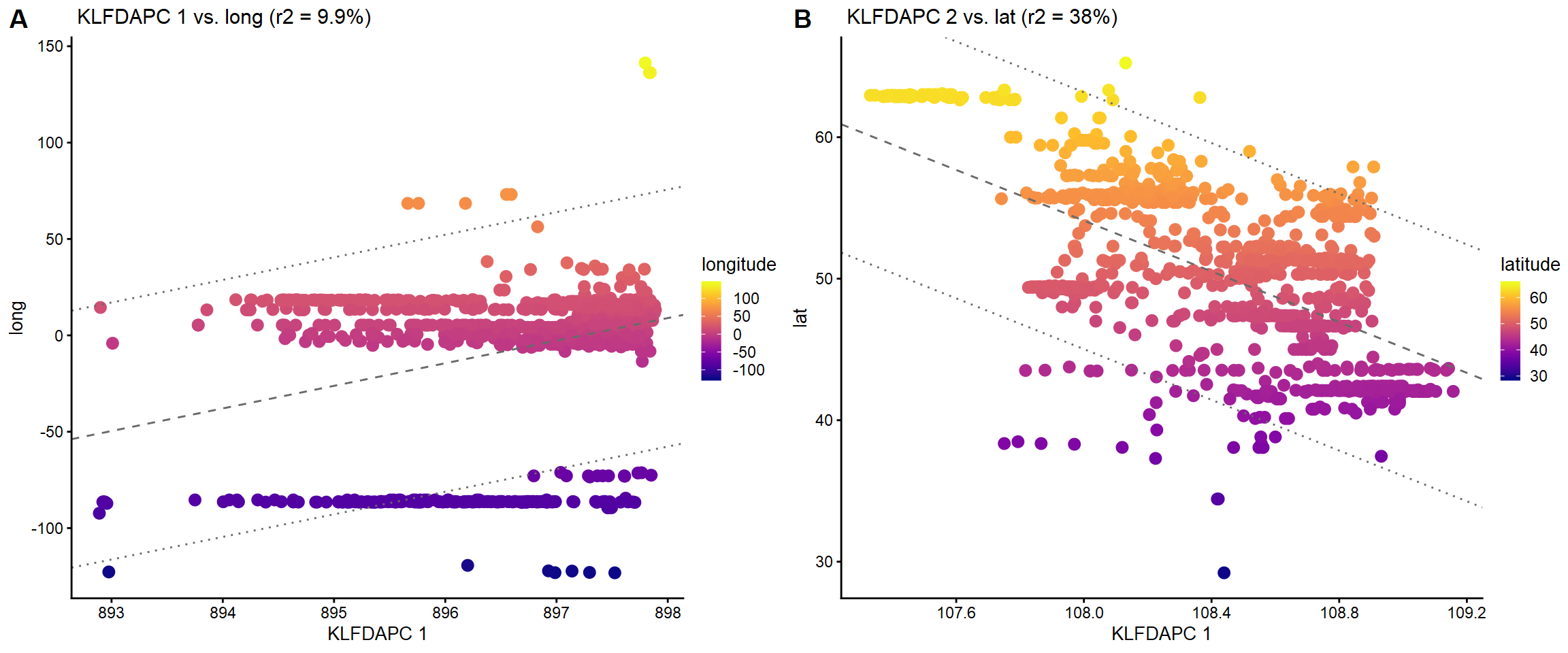
Genetic gradients along longitide and latitude

We would like to see how are the genetic gradients related to geography by looking at the relationships between geography (longitude, latitude) and the genetic gradients.

### Plot the KLFDAPC 2 vs. long
plot1 <- plot(regmapviz1,coord=c("PC1","longitude"),draw.points = TRUE,color = "longitude",group = NULL,plot.title=" KLFDAPC 1 vs. long")+xlab("KLFDAPC 1")+ylab("long")
### Plot the KLFDAPC 2 vs. lat
plot2 <- plot(regmapviz1,coord=c("PC2","latitude"),draw.points = TRUE,color = "latitude",group = NULL,plot.title=" KLFDAPC 2 vs. lat")+xlab("KLFDAPC 1")+ylab("lat")

plot_grid(plot1,plot2,labels = c("A","B"))

Reference

Horton, M. W., Hancock, A. M., Huang, Y. S., Toomajian, C., Atwell, S., Auton, A., … & Nordborg, M. (2012). Genome-wide patterns of genetic variation in worldwide Arabidopsis thaliana accessions from the RegMap panel. Nature genetics, 44(2), 212-216.

Qin, X. 2020. KLFDAPC: Kernel Local Fisher Discriminant Analysis of Principal Components (KLFDAPC) for large genomic data. R package version 0.2.0.

Qin, X., Chiang, C.W.K., and Gaggiotti, O.E. (2021). Kernel Local Fisher Discriminant Analysis of Principal Components (KLFDAPC) significantly improves the accuracy of predicting geographic origin of individuals. bioRxiv, 2021.2005.2015.444294.